Analysis types
Wiring pattern
Every solver follows the same pattern. The screenshots in this section use a small static stress setup: a 120 × 30 × 12 mm aluminum plate with a hole, fixed at one end and loaded with 2000 N at the other.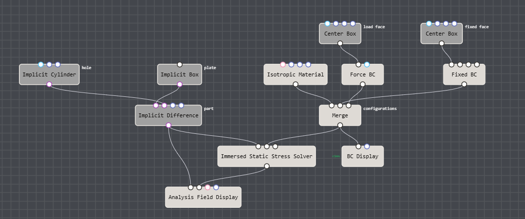
The complete setup. The part goes into the solver's geometry input, the material and boundary conditions are merged into configurations, and the result feeds an Analysis Field Display.
Geometry
Materials and boundary conditions
Merge node and connect it to configurations. Each solver picks the configurations it understands and ignores the rest.Material nodes have a preset list that fills in the properties for common materials. Pick Custom to enter your own values.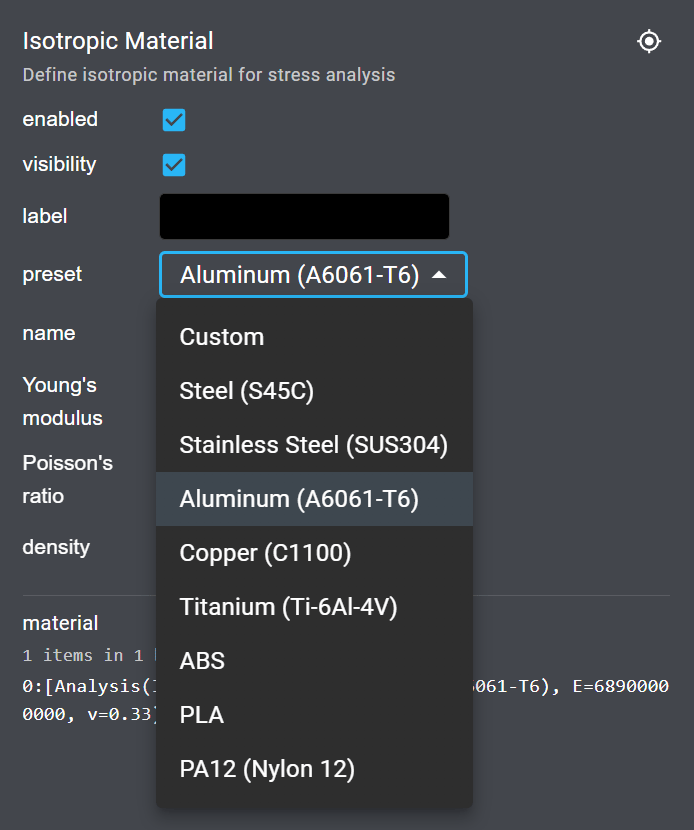
ForceBC takes the total force as a vector, which is distributed over its region.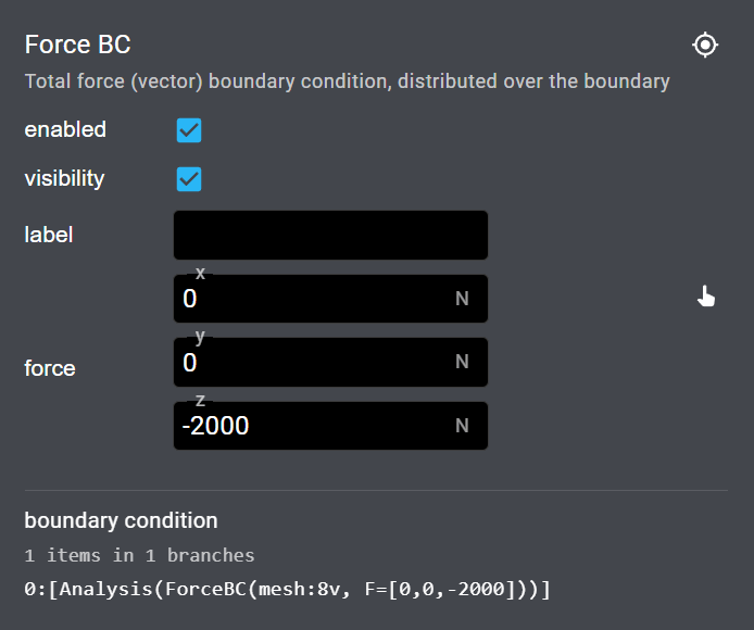
Boundary regions
BrepSelect selection as the region they apply to. A box placed over a face is the quickest way to define a load or support patch. Patches must coincide with a real surface of the domain. For flow inlets and outlets, use the faces of the bounds box.Connect the merged configurations to a BCDisplay node to check the regions in the viewport before you solve.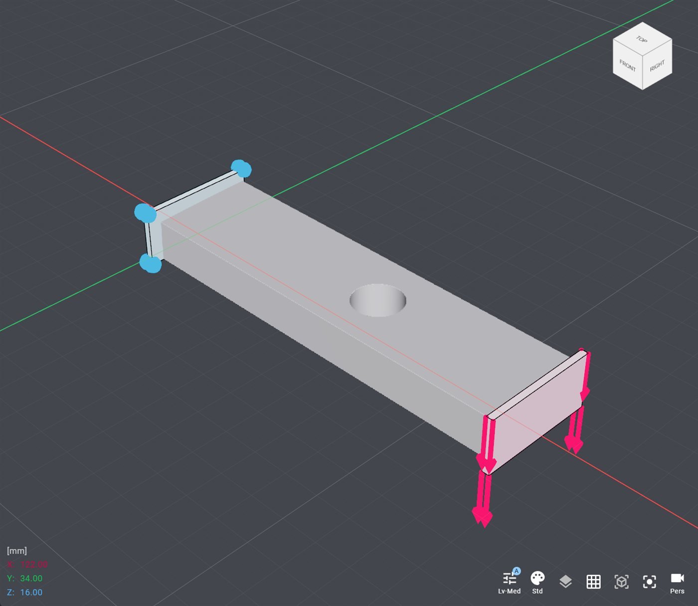
Two thin Center Box regions over the end faces. BCDisplay marks the fixed face with blue markers and the loaded face with arrows in the load direction.
Resolution
- tolerance 4 mm
- tolerance 1 mm
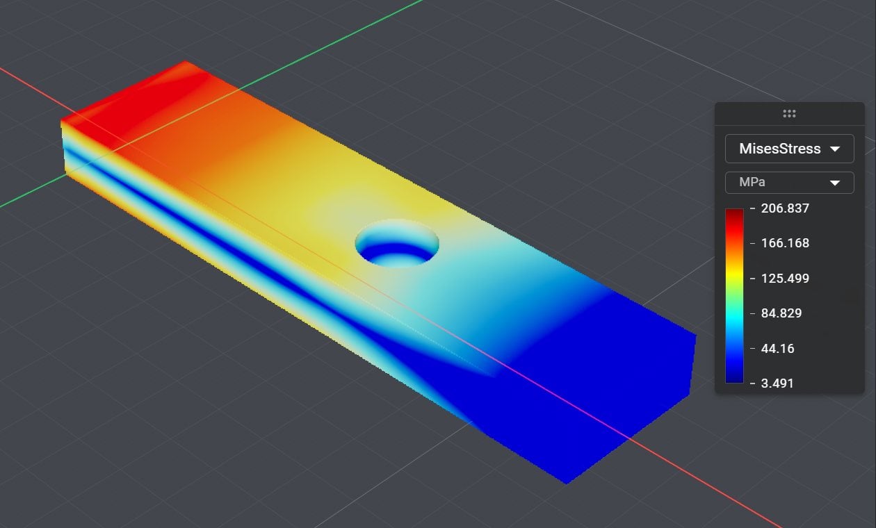
Coarse grid. The overall bending stress is there, but the stress concentration at the hole is missing.
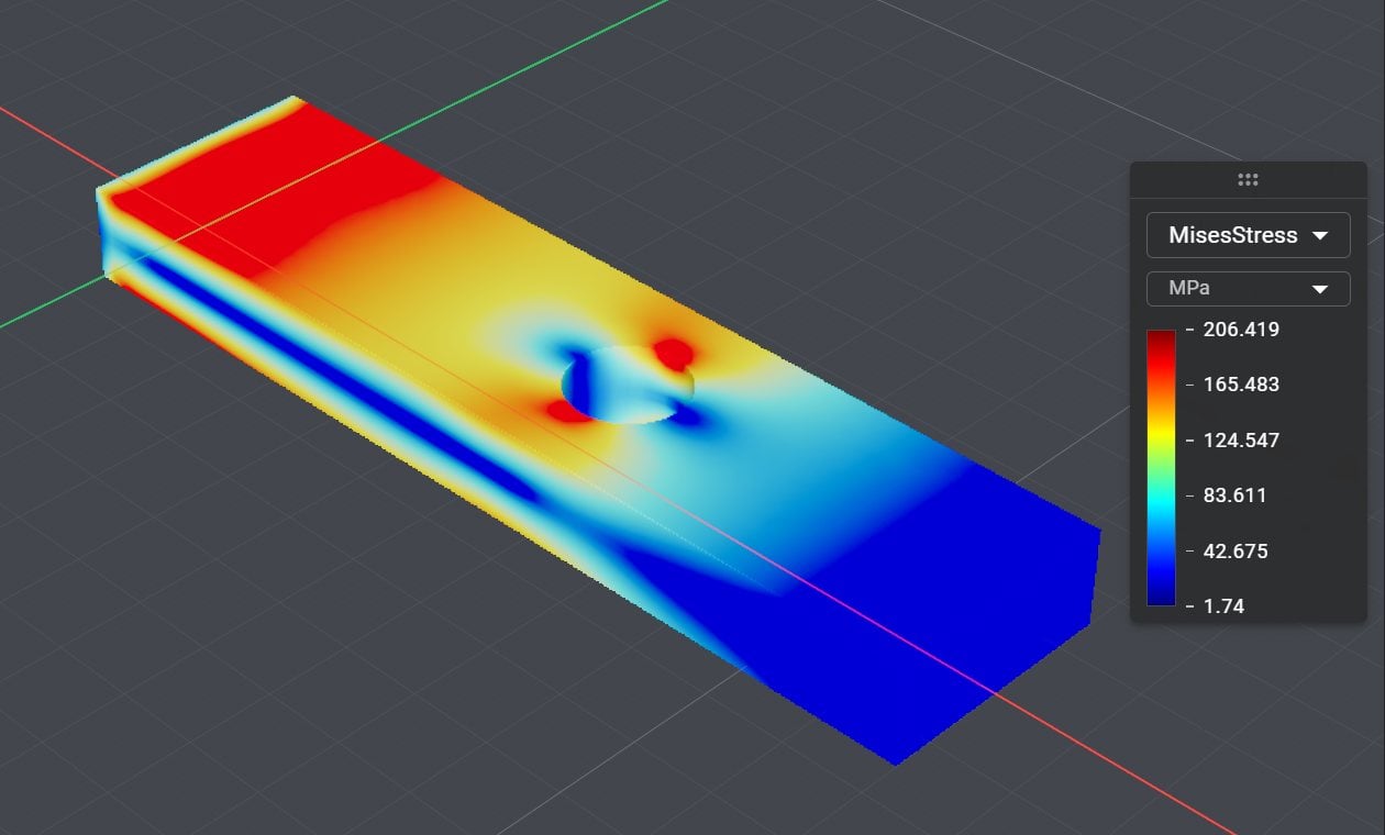
Read the result
FieldSelect to pick one by name, then AnalysisFieldDisplay to shade the part by it, StreamlinesDisplay or FlowParticlesDisplay for velocity fields, and FieldProbe to read values at points. FieldToImplicit and VolumeMeshToImplicit turn results back into geometry.The legend of AnalysisFieldDisplay also has a dropdown that switches between the fields the solver returned, and a unit selector.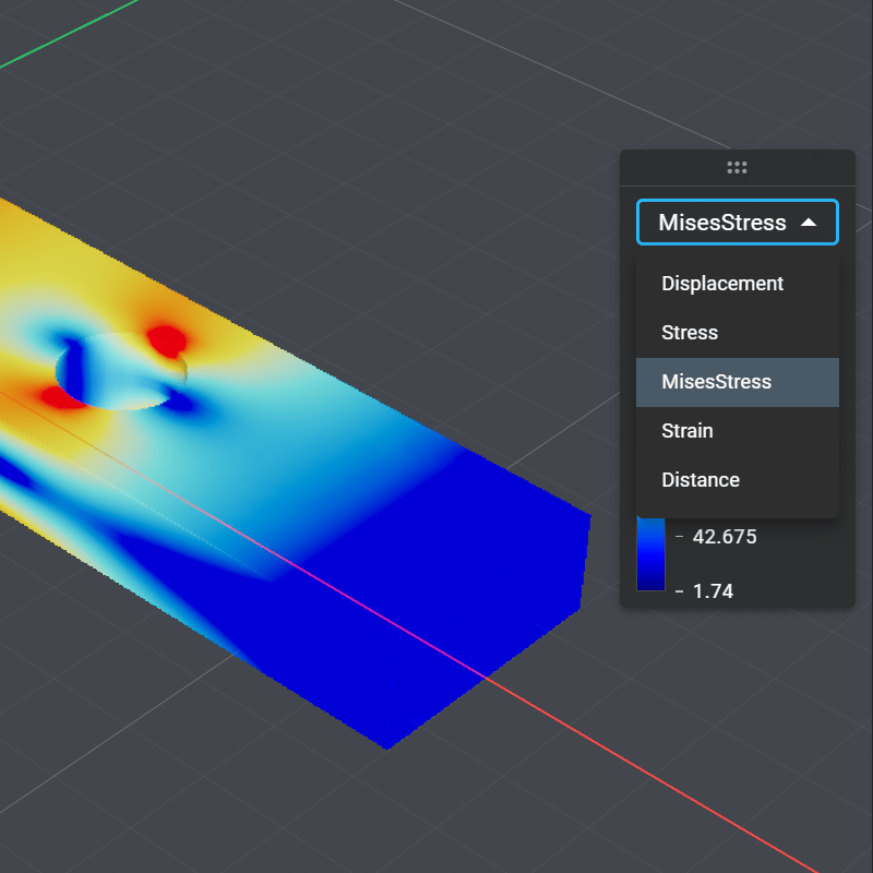
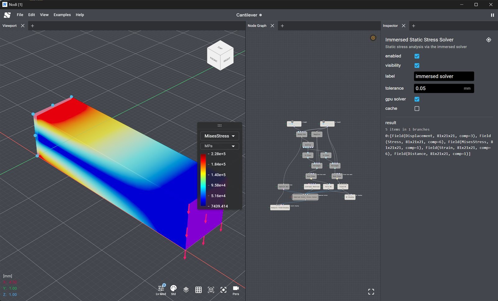
The Cantilever example: the solver node is selected, so the Inspector shows its tolerance, gpu solver and cache properties and the list of result fields.
Flow and thermal analysis
Flow and thermal solvers use the same wiring with their own materials and boundary conditions. In the Channel Flow example, the geometry is the fluid volume of a channel with a spherical obstacle cut out.InletBC drives the flow with a prescribed velocity (or a pressure, selected with drive), OutletBC sets the outflow, and StreamlinesDisplay draws the velocity field.
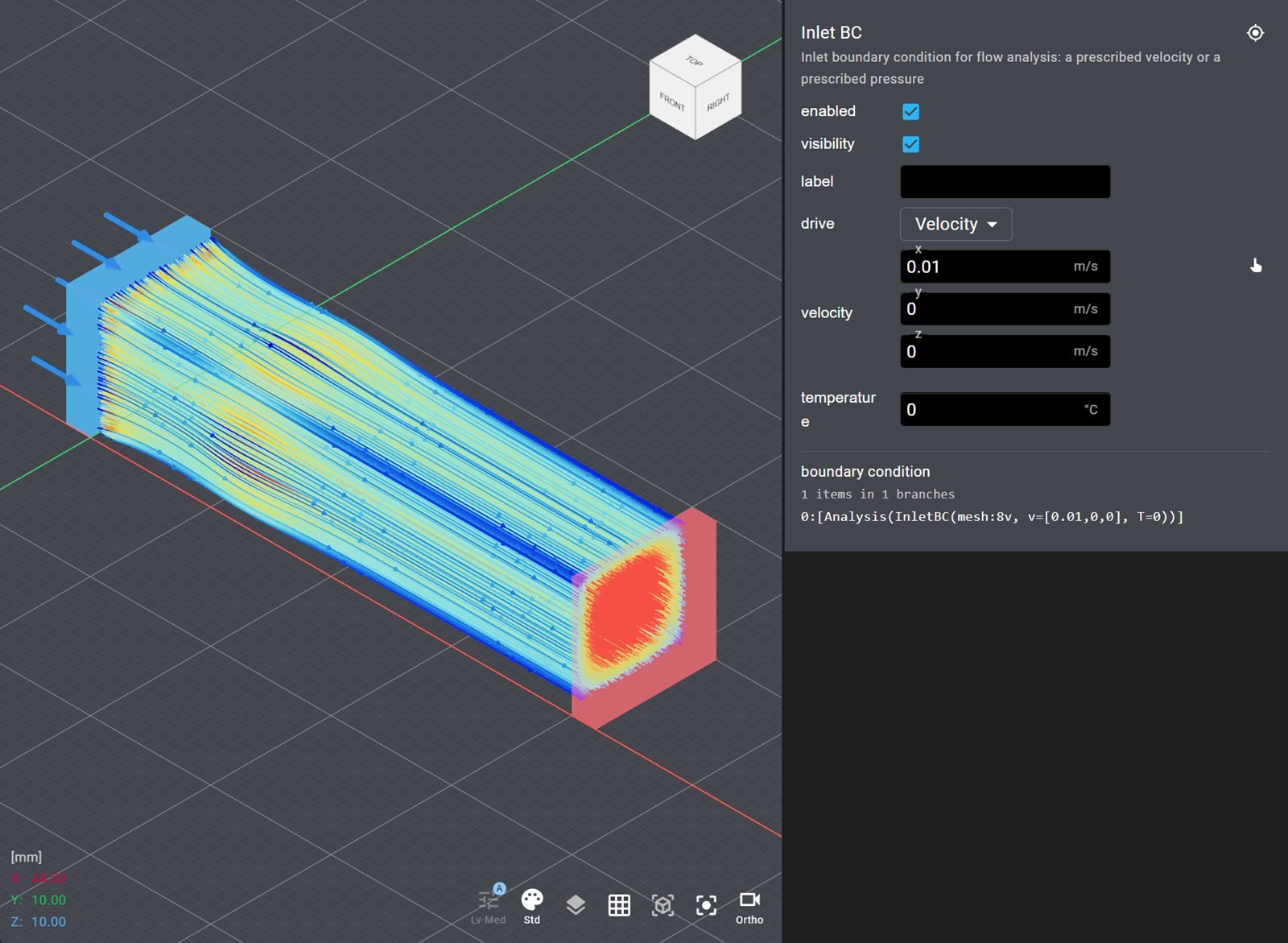
Channel Flow: the inlet patch with its flow direction (blue), the outlet patch (red) and streamlines around the obstacle. The Inspector shows the Inlet BC node.
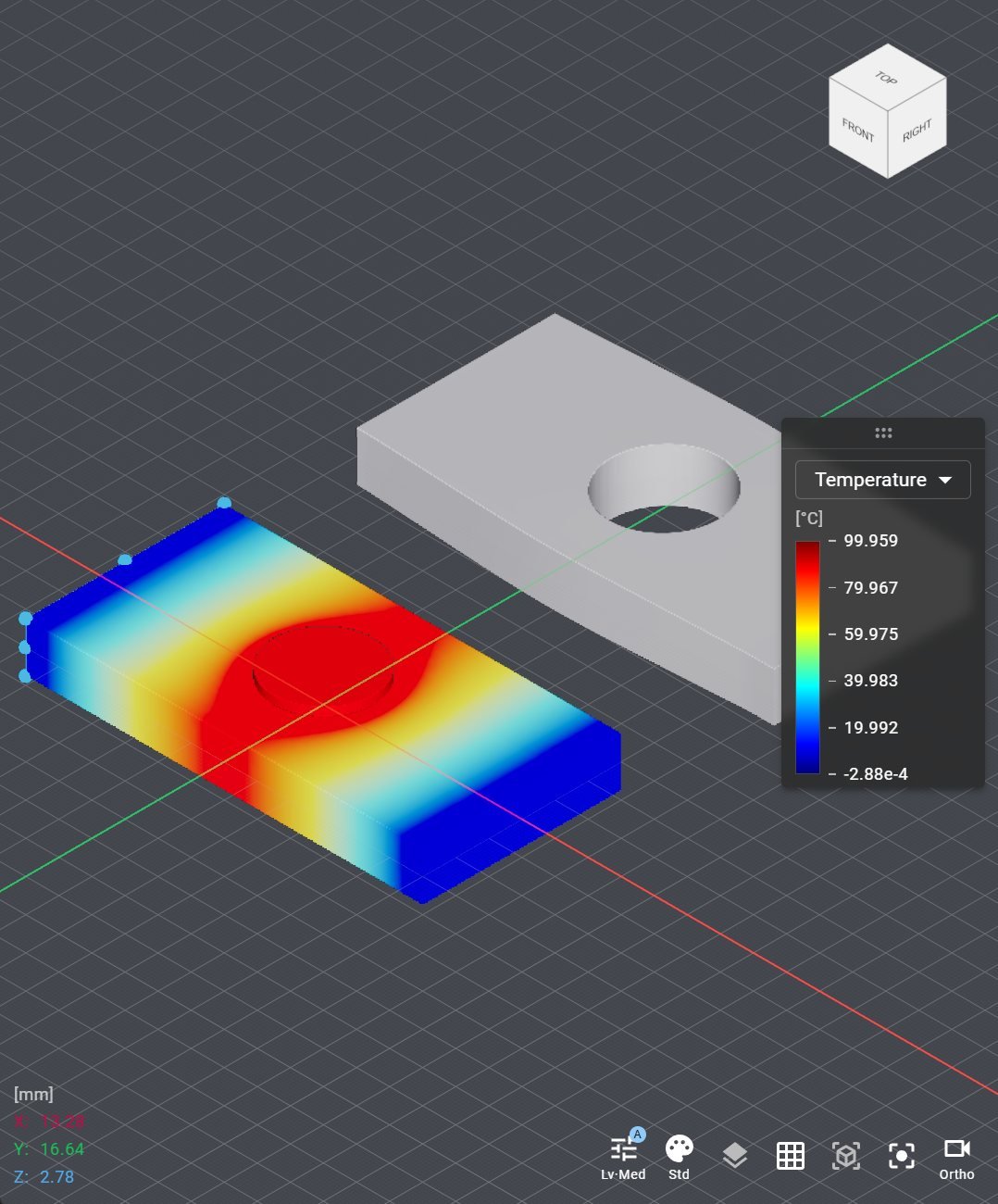
ImmersedStaticThermalStressSolver. The solver returns the temperature together with the stress fields, so the same legend switches between them.
Topology optimization
ImmersedTopologyOptimizer takes a design domain, the same materials and boundary conditions as the analyses above, and a TopologyOptimizationConfig node that selects the method (density or level-set), the objective (compliance, stress, thermal, flow or temperature) and the volume fraction. Connect passive regions to keep areas solid, for example around bolt holes. The node outputs the result fields and an optimized mesh.
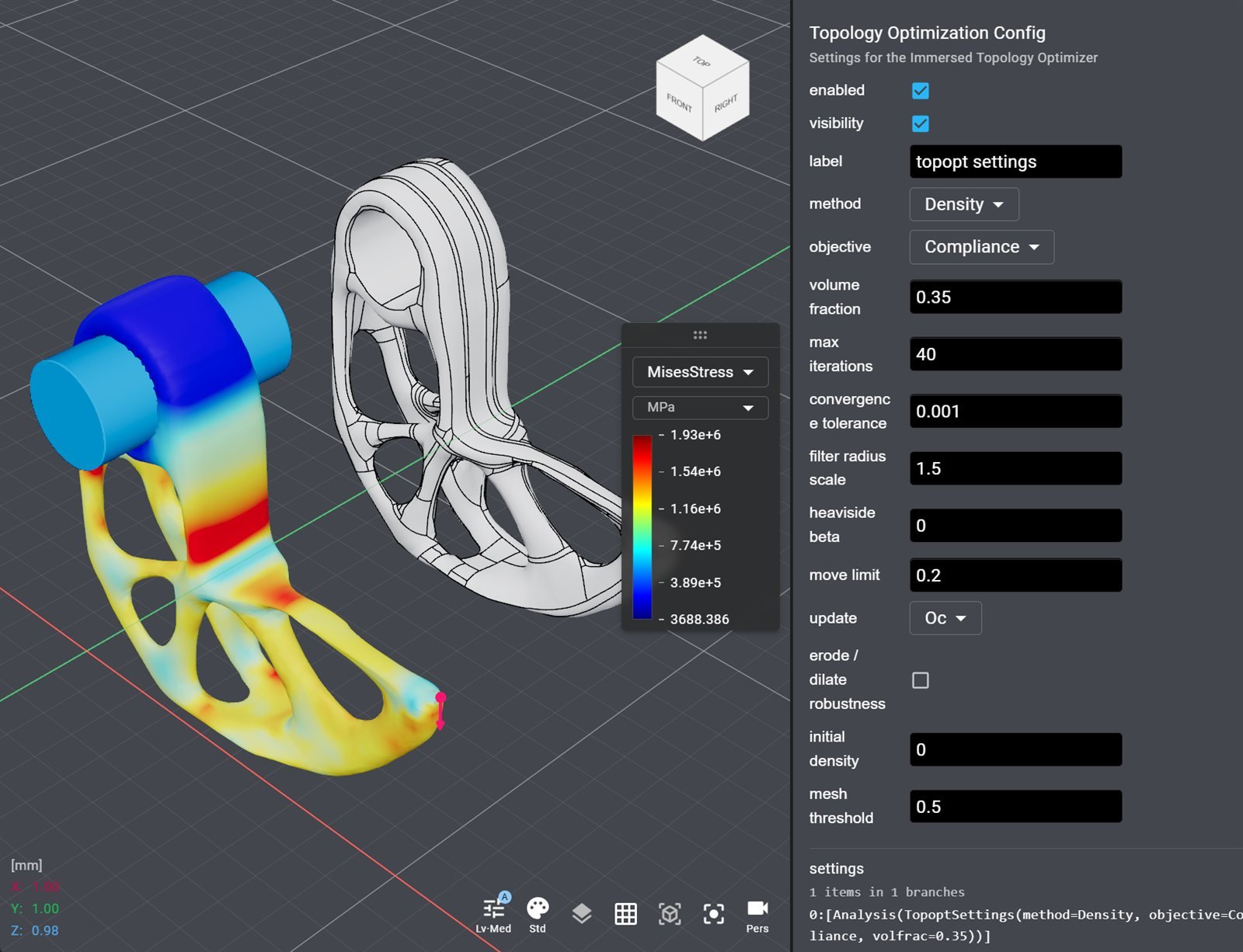
The L-Bracket example: the optimized bracket shaded by Mises stress next to its design, with the Topology Optimization Config node in the Inspector.
Performance
While a solver runs, the viewport shows its progress: the iteration count, the residual against its target and the elapsed time. Click Cancel at the bottom of the node graph to stop a long solve.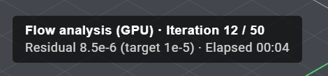
- Enable the gpu solver property when Environment in the app reports GPU Acceleration as available.
- Turn on the node’s cache property and File → Cache so a saved project reopens with its solver results instead of recomputing them.
- One solve runs at a time. Several solver nodes in one graph evaluate one after another.
Examples